How to Prepare a Broad Working Capital or Cash Flows Budget

Breweedes

Editor

posted on 10 years ago — updated on 1 second ago

1
views

In this article you will learn to prepare both a broadly defined working capital budget and a cash flows budget, the latter based on the direct method. In general, working capital is defined as current assets less current liabilities. However, the accounting principles board (APB) of the American Institute of Certified Public Accountants (AICPA) in its Opinion No. 3 broadened the scope of a funds concept from working capital to all financial resources of the firm. Transactions such as giving a mortgage for the acquisition of a plant and/or property, possibly with a cash down payment, would thus be included in their definition of a statement of working capital, whereas this article's intent is rather to prepare an internal budget. Nevertheless, the broader definition is useful, as it includes major transactions that otherwise might be hidden from interested parties such as bankers and investors were such an internal document to be presented as part of a business plan.

Steps

Preparation

Open a new workbook in Excel from the desktop, from the dock, or from your applications folder inside the Microsoft folder. Double click on Excel (either the green X on the dock or the app title in the folder) and select File New Workbook.

In Preferences, in General, set R1C1 to unchecked or Off; in Ribbon, set Ribbon to checked or On; and in View, set Show Formula Bar by Default to checked or On.

Click in the far-upper-left corner above the 1 of row 1 and to the left of column A. Doing so will select the entire worksheet. Format the number of cells to decimal places 0, show comma. Format Cells Font size to 9,10 or 12, bold. Color the cells the lightest sky blue. Title the worksheet, "BudgetWrkgCapital" and save the workbook as "BudgWkgCap" into an appropriate folder such as 'wikiHow Articles'.

Select columns A:C and Format Column Width .3"; select column D and Format Column Width 4.2", select column E:F and Format Column Width 1.75" and Format Cells Number Custom $#,###;$(#,###);$0

The Tutorial: Working Capital Budget - broadly defined

Enter the Statement Header in column E:

Enter (Amounts in Thousands) in cell F1 (if and as applicable), and Format Cells Alignment Center

Enter the Company Name in cell A2: XYZ Corporation

Enter in cell A3: Budget of Working Capital - broadly defined

Enter in cell A4: for the year ending, December 31, 2015 (or as applicable for the current fiscal planning year.)

Enter the line titles and line amounts

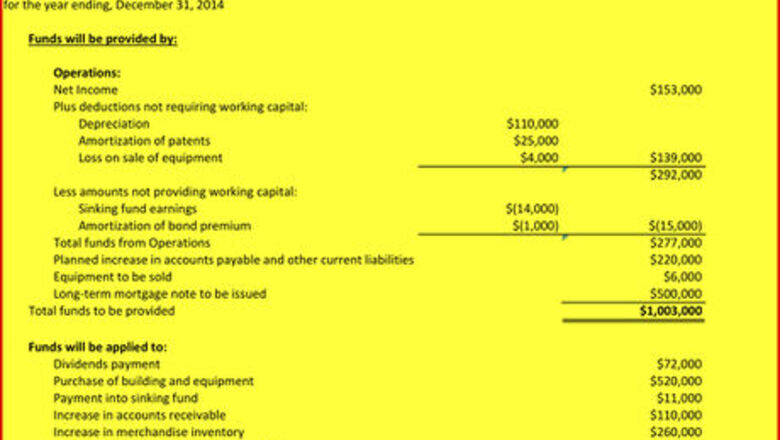
Enter in cell B6: Funds will be provided by:, and Format Cells, Font bold and underlined Enter in cell C8: Operations Enter in cell C9: Net Income Enter in cell C10: Plus deductions not requiring working capital Enter in cell D11: Depreciation Enter in cell D12: Amortization of patents Enter in cell D13: Loss on sale of equipment Enter in cell F9: 153000 Enter in cell E11: 110000 Enter in cell E12: 25000 Enter in cell E13: 4000 and Format Cells Border underline Enter in cell F13: the formula =SUM(E11:E13) (, result = $139,000) and Format Cells Border underline Enter in cell F14: the formula =SUM(F9:F13) (, result = $292,000) Enter in cell C15: Less amounts not providing working capital: Enter in cell D16: Sinking fund earnings Enter in cell D17: Amortization of bond premium Enter in cell C18: Total funds from Operations Enter in cell E16: -14000 Enter in cell E17: -1000 and Format Cells Border underline Enter in cell F17: the formula =SUM(E16:E17) and Format Cells Border underline (, result = $15,000) Enter in cell F18: the formula =SUM(F14:F17) (, result = $277,000) Enter in cell C19: Planned increase in accounts payable and other current liabilities Enter in cell F19: 220000 Enter in cell C20: Equipment to be sold Enter in cell F20: 6000 Enter in cell C21: Long-term mortgage note to be issued Enter in cell F21: 500000 and Format Cells Border underline Enter in cell B22: Total funds to be provided Enter in cell F22: the formula =SUM(F18:F21) and Format Cells Border DOUBLE underline and bold (, result = $1,003,000)

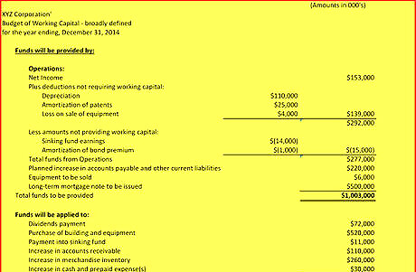
Enter in cell B24: Funds will be applied to: and Format Cells bold Enter in cell C25: Dividends payment Enter in cell C26: Purchase of building and equipment Enter in cell C27: Payment into sinking fund Enter in cell C28: Increase in accounts receivable Enter in cell C29: Increase in merchandise inventory Enter in cell C30: Increase in cash and prepaid expense(s) Enter in cell F25: 72000 Enter in cell F26: 520000 Enter in cell F27: 11000 Enter in cell F28: 110000 Enter in cell F29: 260000 Enter in cell F30: 30000 and Format Cells underline Enter to cell B31: Total funds to be applied Enter to cell F31: the formula, =SUM(F25:F30) and Format Cells Border DOUBLE underline and bold (, result = $1,003,000) Your Working Capital Budget should resemble the one pictured here if you apply a canary yellow to all the cells.

The Tutorial: Cash Flows Budget - Direct Method

Title the next worksheet tab, CashFlowsBudget

Select columns A:B and Format column width, .3"

Select column C and Format column width 4"

Enter to cell A1: Cash Flows Budget, XYZ Corporation

Enter to cell A2: for the year ended December 31, 2015 (or as applicable for the current fiscal planning year)

Enter to cell E1: (000's) and Format Cells Alignment Center

Select columns D:E and Format Cells Number Custom $#,###;$(#,###);$0

Enter the line items and amounts Enter to cell A4: Cash flows to be used in (from) operating activities, and Format Cells bold Enter to cell B5: Cash receipts from customers Enter to cell B6: Cash paid to suppliers and employees Enter to cell B7: Equals: Cash generated from operations Enter to cell D5: 10000 Enter to cell D6: -2500 and Format Cells Border underline Enter to cell E7: the formula =SUM(D5:D6) Enter to cell B8: Interest payments Enter to cell B9: Income tax payments and Format Cells Border underline Enter to cell C10: Net cash flows from operating activities Enter to cell D8: -2100 Enter to cell D9: -2600 and Format Cells Border underline Enter to cell E9: the formula =SUM(D8:D9), and Format Cells Border underline Enter to cell E10: the formula =SUM(E7:E9)

Enter to cell A12: Cash flows to be used in (from) investing activities, and Format Cells bold Enter to cell B13: Equipment to be sold Enter to cell B14: Dividend Receipts Enter to cell C15: Net cash flows from investing activities Enter to cell D13: 8500 Enter to cell D14: 3000 and Format Cells Border underline Enter to cell E15: the formula =SUM(D13:D14)

Enter to cell A17: Cash flows to be used in (from) financing activities, and Format Cells bold Enter to cell B18: Dividend payments Enter to cell C19: Net cash flows from financing activities Enter to cell D18: -2800 and Format Cells Border underline Enter to cell E19: the formula =D18

Enter to cell A21: Net increase in cash and cash equivalents planned Enter to cell E21: the formula =SUM(E10:E20)

Enter to cell A22: Cash and cash equivalents, beginning of fiscal planning year Enter to cell E22: 1150

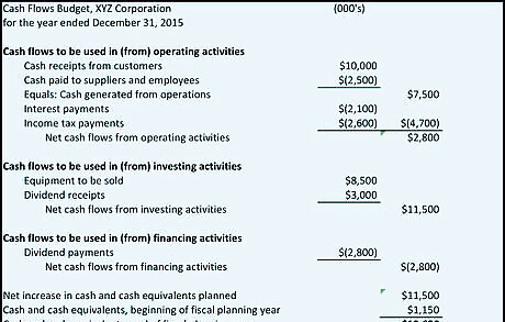
Enter to cell A23: Cash and cash equivalents, end of fiscal planning year Enter to cell E23: the formula =SUM(E21:E22), and Format Cells bold and DOUBLE underline border. Your cash flows budget should resemble the one pictured here if you apply a light blue to all the cells.