views
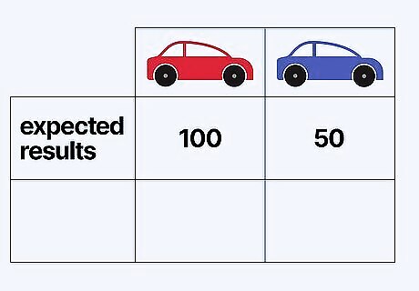
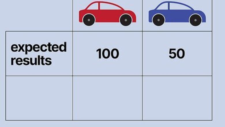
Determine your experiment's expected results. Usually, when scientists conduct an experiment and observe the results, they have an idea of what "normal" or "typical" results will look like beforehand. This can be based on past experimental results, trusted sets of observational data, scientific literature, and/or other sources. For your experiment, determine your expected results and express them as a number. Example: Let's say prior studies have shown that, nationally, speeding tickets are given more often to red cars than they are to blue cars. Let's say the average results nationally show a 2:1 preference for red cars. We want to find out whether or not the police in our town also demonstrate this bias by analyzing speeding tickets given by our town's police. If we take a random pool of 150 speeding tickets given to either red or blue cars in our town, we would expect 100 to be for red cars and 50 to be for blue cars if our town's police force gives tickets according to the national bias.
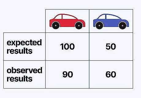
Determine your experiment's observed results. Now that you've determined your expected values, you can conduct your experiment and find your actual (or "observed") values. Again, express these results as numbers. If we manipulate some experimental condition and the observed results differ from this expected results, two possibilities are possible: either this happened by chance, or our manipulation of experimental variables caused the difference. The purpose of finding a p-value is basically to determine whether the observed results differ from the expected results to such a degree that the "null hypothesis" - the hypothesis that there is no relationship between the experimental variable(s) and the observed results - is unlikely enough to reject. Example: Let's say that, in our town, we randomly selected 150 speeding tickets which were given to either red or blue cars. We found that 90 tickets were for red cars and 60 were for blue cars. These differ from our expected results of 100 and 50, respectively. Did our experimental manipulation (in this case, changing the source of our data from a national one to a local one) cause this change in results, or are our town's police as biased as the national average suggests, and we're just observing a chance variation? A p value will help us determine this.
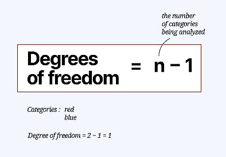
Determine your experiment's degrees of freedom. Degrees of freedom are a measure the amount of variability involved in the research, which is determined by the number of categories you are examining. The equation for degrees of freedom is Degrees of freedom = n-1, where "n" is the number of categories or variables being analyzed in your experiment. Example: Our experiment has two categories of results: one for red cars and one for blue cars. Thus, in our experiment, we have 2-1 = 1 degree of freedom. If we had compared red, blue, and green cars, we would have 2 degrees of freedom, and so on.
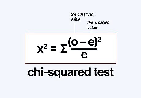
Compare expected results to observed results with chi square. Chi square(written "x") is a numerical value that measures the difference between an experiment's expected and observed values. The equation for chi square is: x = Σ((o-e)/e), where "o" is the observed value and "e" is the expected value. Sum the results of this equation for all possible outcomes (see below). Note that this equation includes a Σ (sigma) operator. In other words, you'll need to calculate ((|o-e|-.05)/e) for each possible outcome, then add the results to get your chi square value. In our example, we have two outcomes - either the car that received a ticket is red or blue. Thus, we would calculate ((o-e)/e) twice - once for red cars and once for blue cars. Example: Let's plug our expected and observed values into the equation x = Σ((o-e)/e). Keep in mind that, because of the sigma operator, we'll need to perform ((o-e)/e) twice - once for red cars and once for blue cars. Our work would go as follows: x = ((90-100)/100) + (60-50)/50) x = ((-10)/100) + (10)/50) x = (100/100) + (100/50) = 1 + 2 = 3 .
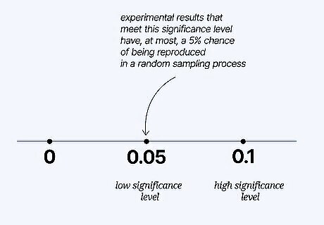
Choose a significance level. Now that we know our experiment's degrees of freedom and our chi square value, there's just one last thing we need to do before we can find our p value - we need to decide on a significance level. Basically, the significance level is a measure of how certain we want to be about our results - low significance values correspond to a low probability that the experimental results happened by chance, and vice versa. Significance levels are written as a decimal (such as 0.01), which corresponds to the percent chance that random sampling would produce a difference as large as the one you observed if there was no underlying difference in the populations. It is a common misconception that p=0.01 means that there is a 99% chance that the results were caused by the scientist's manipulation of experimental variables. This is NOT the case. If you wore your lucky pants on seven different days and the stock market went up every one of those days, you would have p<0.01, but you would still be well-justified in believing that the result had been generated by chance rather than by a connection between the market and your pants. By convention, scientists usually set the significance value for their experiments at 0.05, or 5 percent. This means that experimental results that meet this significance level have, at most, a 5% chance of being reproduced in a random sampling process. For most experiments, generating results that are that unlikely to be produced by a random sampling process is seen as "successfully" showing a correlation between the change in the experimental variable and the observed effect. Example: For our red and blue car example, let's follow scientific convention and set our significance level at 0.05.
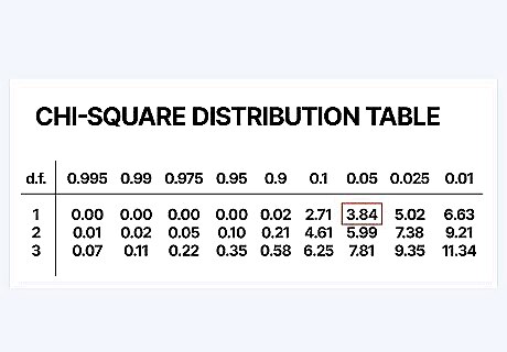
Use a chi square distribution table to approximate your p-value. Scientists and statisticians use large tables of values to calculate the p value for their experiment. These tables are generally set up with the vertical axis on the left corresponding to degrees of freedom and the horizontal axis on the top corresponding to p-value. Use these tables by first finding your degrees of freedom, then reading that row across from the left to the right until you find the first value bigger than your chi square value. Look at the corresponding p value at the top of the column - your p value is between this value and the next-largest value (the one immediately to the left of it). Chi square distribution tables are available from a variety of sources - they can easily be found online or in science and statistics textbooks. If you don't have one handy, use the one in the photo above or a free online table, like the one provided by medcalc.org here. Example: Our chi-square was 3. So, let's use the chi square distribution table in the photo above to find an approximate p value. Since we know our experiment has only 1 degree of freedom, we'll start in the highest row. We'll go from left to right along this row until we find a value higher than 3 - our chi square value. The first one we encounter is 3.84. Looking to the top of this column, we see that the corresponding p value is 0.05. This means that our p value is between 0.05 and 0.1 (the next-biggest p value on the table).
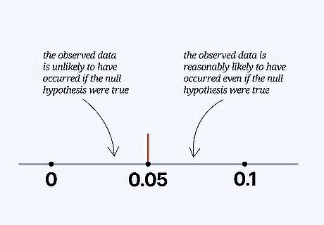
Decide whether to reject or keep your null hypothesis. Since you have found an approximate p value for your experiment, you can decide whether or not to reject the null hypothesis of your experiment (as a reminder, this is the hypothesis that the experimental variables you manipulated did not affect the results you observed.) If your p value is lower than your significance value, congratulations - you've shown that your experimental results would be highly unlikely to occur if there was no real connection between the variables you manipulated and the effect you observed. If your p value is higher than your significance value, you can't confidently make that claim. Example: Our p value is between 0.05 and 0.1 . It is not smaller than 0.05, so, unfortunately, we can't reject our null hypothesis. This means that we didn't reach the criterion we decided upon to be able to say that our town's police give tickets to red and blue cars at a rate that's significantly different than the national average. In other words, random sampling from the national data would produce a result 10 tickets off from the national average 5-10% of the time. Since we were looking for this percentage to be less than 5%, we can't say that we're sure our town's police are less biased towards red cars.





Comments
0 comment