How to Calculate Outliers

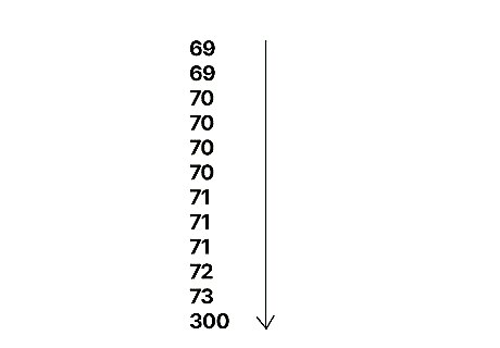
Arrange all data points from lowest to highest. The first step when calculating outliers in a data set is to find the median (middle) value of the data set. This task is greatly simplified if the values in the data set are arranged in order of least to greatest. So, before continuing, sort the values in your data set in this fashion. Let's continue with the example above. Here is our data set representing the temperatures of several objects in a room: {71, 70, 73, 70, 70, 69, 70, 72, 71, 300, 71, 69}. If we order the values in the data set from lowest to highest, our new set of values is: {69, 69, 70, 70, 70, 70, 71, 71, 71, 72, 73, 300}.

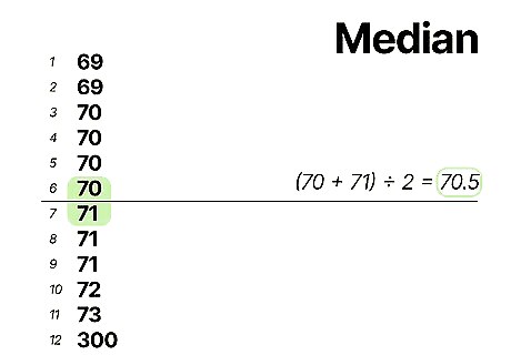
Calculate the median of the data set. The median of a data set is the data point above which half of the data sits and below which half of the data sits - essentially, it's the "middle" point in a data set. If the data set contains an odd number of points, this is easy to find - the median is the point which has the same number of points above as below it. However, if there are an even number of points, then, since there is no single middle point, the 2 middle points should be averaged to find the median. Note that, when calculating outliers, the median is usually assigned the variable Q2 - - this is because it lies between Q1 and Q3, the lower and upper quartiles, which we will define later. Don't be confused by data sets with even numbers of points - the average of the two middle points will often be a number that doesn't appear in the data set itself - this is OK. However, if the two middle points are the same number, the average, obviously, will be this number as well, which is also OK. In our example, we have 12 points. The middle 2 terms are points 6 and 7 - 70 and 71, respectively. So, the median for our data set is the average of these two points: ((70 + 71) / 2), = 70.5.

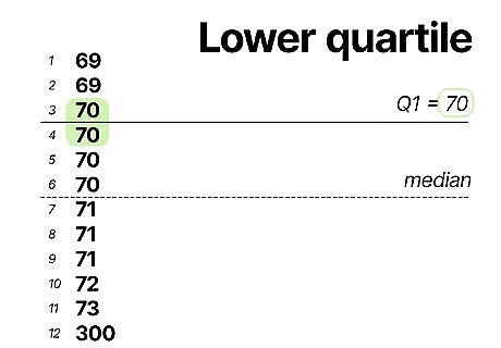
Calculate the lower quartile. This point, to which we will assign the variable Q1, is the data point below which 25 percent (or one quarter) of the observations set. In other words, this is the halfway point of the points in your data set below the median. If there are an even number of values below the median, you once again must average the two middle values to find Q1, much like you may have had to do to find the median itself. In our example, 6 points lie above the median and 6 points lie below it. This means that, to find the lower quartile, we will need to average the two middle points of the bottom six points. Points 3 and 4 of the bottom 6 are both equal to 70. Thus, their average is ((70 + 70) / 2), = 70. 70 will be our value for Q1

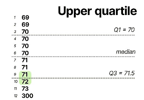
Calculate the upper quartile. This point, which is assigned the variable Q3, is the data point above which 25 percent of the data sits. Finding Q3 is almost identical to finding Q1, except that, in this case, the points above the median, rather than below it, are taken into account. Continuing with the example above, the two middle points of the 6 points above the median are 71 and 72. Averaging these 2 points gives ((71 + 72) / 2), = 71.5. 71.5 will be our value for Q3.

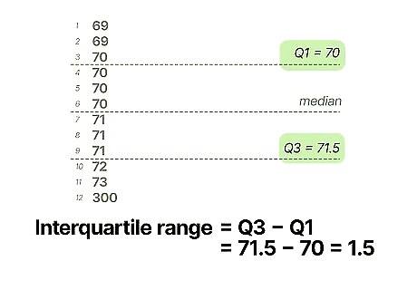
Find the interquartile range. Now that we've defined Q1 and Q3, we need to calculate the distance between these two variables. The distance from Q1 to Q3 is found by subtracting Q1 from Q3. The value you obtain for the interquartile range is vital for determining the boundaries for non-outlier points in your data set. In our example, our values for Q1 and Q3 are 70 and 71.5, respectively. To find the interquartile range, we subtract Q3 - Q1: 71.5 - 70 = 1.5. Note that this works even if Q1, Q3, or both are negative numbers. For example, if our Q1 value was -70, our interquartile range would be 71.5 - (-70) = 141.5, which is correct.

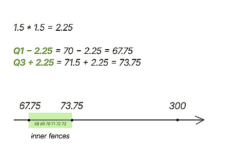
Find the "inner fences" for the data set. Outliers are identified by assessing whether or not they fall within a set of numerical boundaries called "inner fences" and "outer fences". A point that falls outside the data set's inner fences is classified as a minor outlier, while one that falls outside the outer fences is classified as a major outlier. To find the inner fences for your data set, first, multiply the interquartile range by 1.5. Then, add the result to Q3 and subtract it from Q1. The two resulting values are the boundaries of your data set's inner fences. In our example, the interquartile range is (71.5 - 70), or 1.5. Multiplying this by 1.5 yields 2.25. We add this number to Q3 and subtract it from Q1 to find the boundaries of the inner fences as follows: 71.5 + 2.25 = 73.75 70 - 2.25 = 67.75 Thus, the boundaries of our inner fence are 67.75 and 73.75. In our data set, only the temperature of the oven - 300 degrees - lies outside this range and thus may be a mild outlier. However, we have yet to determine if this temperature is a major outlier, so let's not draw any conclusions until we do so.

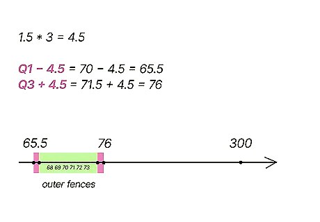
Find the "outer fences" for the data set. This is done in the same way as the inner fences, except that the interquartile range is multiplied by 3 instead of 1.5. The result is then added to Q3 and subtracted from Q1 to find the upper and lower boundaries of the outer fence. In our example, multiplying the interquartile range above by 3 yields (1.5 * 3), or 4.5. We find the boundaries of the outer fence in the same fashion as before: 71.5 + 4.5 = 76 70 - 4.5 = 65.5 The boundaries of our outer fence are 65.5 and 76. Any data points that lie outside the outer fences are considered major outliers. In this example, the oven temperature, 300 degrees, lies well outside the outer fences, so it's definitely a major outlier.

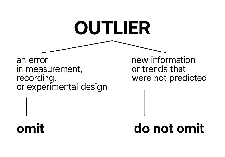
Use a qualitative assessment to determine whether to "throw out" outliers. Using the methodology described above, it's possible to determine whether certain points are minor outliers, major outliers, or not outliers at all. However, make no mistake - identifying a point as an outlier only marks it as a candidate for omission from the data set, not as a point that must be omitted. The reason that an outlier differs from the rest of the points in the data set is crucial in determining whether to omit the outlier or not. Generally, outliers that can be attributed to an error of some sort - an error in measurement, recording, or experimental design, for instance - are omitted. On the other hand, outliers that are not attributed to error and that reveal new information or trends that were not predicted are usually not omitted. Another criterion to consider is whether outliers significantly impact the mean (average) of a data set in a way that skews it or makes it appear misleading. This is especially important to consider if you intend to draw conclusions from the mean of your data set. Let's assess our example. In our example, since it's highly unlikely that the oven reached a temperature of 300 degrees through some unforeseen natural force, we can conclude with near-certainty that the oven was accidentally left on, resulting in the anomalous high temperature reading. Also, if we don't omit the outlier, the mean of our data set is (69 + 69 + 70 + 70 + 70 + 70 + 71 + 71 + 71 + 72 + 73 + 300)/12 = 89.67 degrees, while the mean if we do omit the outlier is (69 + 69 + 70 + 70 + 70 + 70 + 71 + 71 + 71 + 72 + 73)/11 = 70.55. Since the outlier can be attributed to human error and because it's inaccurate to say that this room's average temperature was almost 90 degrees, we should opt to omit our outlier.

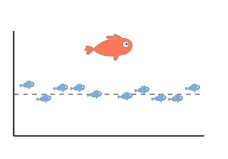
Understand the importance of (sometimes) retaining outliers. While some outliers should be omitted from data sets because they result from error and/or skew results in ways that are inaccurate or misleading, some outliers should be kept. If, for example, an outlier appears to be genuinely obtained (that is, not the result of error) and/or gives some new insight into the phenomenon being measured, they should not be omitted out of hand. Scientific experiments are especially sensitive situations when dealing with outliers - omitting an outlier in error can mean omitting information that signifies some new trend or discovery. For instance, let's say that we're designing a new drug to increase the size of fish in a fish farm. We'll use our old data set ({71, 70, 73, 70, 70, 69, 70, 72, 71, 300, 71, 69}), except, this time, each point will represent the mass of a fish (in grams) after being treated with a different experimental drug from birth. In other words, the first drug gave one fish a mass of 71 grams, the second drug gave a different fish a mass of 70 grams, and so on. In this situation, 300 is still a big outlier, but we shouldn't omit it because, assuming it's not due to an error, it represents a significant success in our experiment. The drug that yielded a 300 gram fish worked better than all the other drugs, so this point is actually the most important one in our data set, rather than the least.

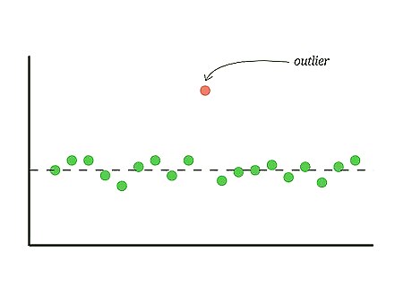
Learn how to recognize potential outliers. Before deciding whether or not to omit outlying values from a given data set, first, obviously, we must identify the data set's potential outliers. Generally speaking, outliers are data points that differ greatly from the trend expressed by the other values in the data set - in other words, they lie outside the other values. It's usually easy to detect this on data tables or (especially) on graphs. If the data set is expressed visually on the graph, outlying points will be "far away" from the other values. If, for instance, the majority of the points in a data set form a straight line, outlying values will not be able to be reasonably construed to conform to the line. Let's consider a data set that represents the temperatures of 12 different objects in a room. If 11 of the objects have temperatures within a few degrees of 70 degrees Fahrenheit (21 degrees Celsius), but the twelfth object, an oven, has a temperature of 300 degrees Fahrenheit (150 degrees Celsius), a cursory examination can tell you that the oven is a likely outlier.