
- An inflection point is where a function changes concavity and where the second derivative of the function changes signs.
- Take the first and second derivative of the function using the power rule.
- Set the second derivative equal to 0 to find the candidate, or possible, inflection points.
- Plug in a value greater than and less than the candidate point to see if the second derivative changes signs at the point.
Understanding Convexity, Concavity and Inflection
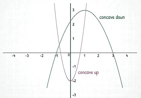
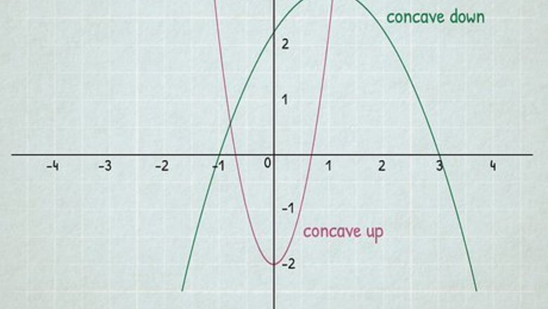
Learn the difference between convex and concave. To understand inflection points, you need to understand when a function is convex or concave on a graph. Many functions have both convex and concave intervals, with an inflection point existing where a function changes convexity/concavity. Luckily, convex and concave are easy to distinguish based on what they look like. A concave function is shaped like a hill or an upside-down U. It’s a function where the slope is decreasing. When it’s graphed, no line segment that joins 2 points on its graph ever goes above the curve. A convex function, on the other hand, is shaped like a U. It’s a function where the slope is increasing. No line segment that joins 2 points on its graph ever goes below the curve. In the graph above, the red curve is convex, while the green curve is concave.
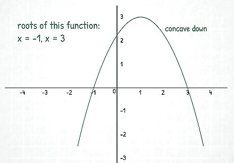
Identify the roots of a function. A root of a function is the point where the function equals zero, or where the function intersects the x-axis. In the graph above, the roots of the green parabola are at x = − 1 {\displaystyle x=-1} x=-1 and x = 3. {\displaystyle x=3.} x=3. A function can also have more than 1 root.
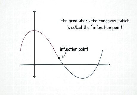
Find an inflection point where a function changes concavity. Remember how there’s a difference between convex and concave? An inflection point is a point on a function where its shape changes, either from convex to concave, or opposite. It is also the point where the second derivative of the function changes signs from positive to negative or negative to positive, thus being equal 0. For a point to be the point of inflection, it has to both switch convexity/concavity and change signs on the second derivative. To find the inflection point on a graph, look for the point where the function switches concavity. On the graph above, it’s the middle point where the function changes from concave to convex.
Finding the Derivatives of a Function
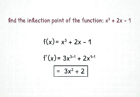
Take the first derivative of the given function. You’ll need your function's second derivative to find your inflection points. Before you get the second derivative, you have to find the first derivative of the function. First derivatives are denoted as f ′ ( x ) {\displaystyle f^{\prime }(x)} f^{{\prime }}(x) or d f d x {\displaystyle {\frac {\mathrm {d} f}{\mathrm {d} x}}} {\frac {{\mathrm {d}}f}{{\mathrm {d}}x}}. To solve your function’s first derivative, use the power rule. Multiply x by its exponent and then reduce the exponent by 1. For example, find the inflection point of the function below. f ( x ) = x 3 + 2 x − 1 {\displaystyle f(x)=x^{3}+2x-1} f(x)=x^{{3}}+2x-1 Use the power rule to find the first derivative. f ′ ( x ) = 3 x 3 − 1 + 2 x 1 − 1 f ′ ( x ) = 3 x 2 + 2 {\displaystyle {\begin{aligned}f^{\prime }(x)&=3x^{3-1}+2x^{1-1}\\f^{\prime }(x)&=3x^{2}+2\end{aligned}}} {\displaystyle {\begin{aligned}f^{\prime }(x)&=3x^{3-1}+2x^{1-1}\\f^{\prime }(x)&=3x^{2}+2\end{aligned}}} The derivatives of basic functions are usually found in most calculus textbooks; you need to learn how to find basic derivatives before moving on to more complex functions.
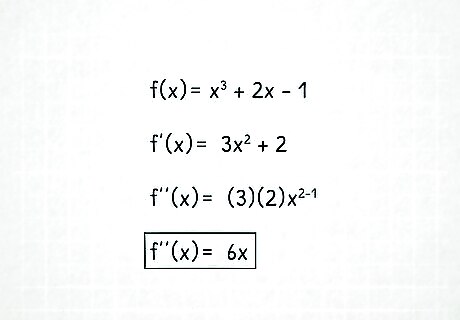
Differentiate the function again to get the second derivative. The second derivative is the derivative of the first derivative. It is denoted as f ′ ′ ( x ) {\displaystyle f^{\prime \prime }(x)} f^{{\prime \prime }}(x) or d 2 f d x 2 . {\displaystyle {\frac {\mathrm {d} ^{2}f}{\mathrm {d} x^{2}}}.} {\frac {{\mathrm {d}}^{{2}}f}{{\mathrm {d}}x^{{2}}}}. Simply use the power rule again to get the second derivative. Find the second derivative of f ′ ( x ) = 3 x 2 + 2 {\displaystyle {\begin{aligned}f^{\prime }(x)&=3x^{2}+2\end{aligned}}} {\displaystyle {\begin{aligned}f^{\prime }(x)&=3x^{2}+2\end{aligned}}} f ′ ′ ( x ) = ( 2 ) ( 3 ) x 2 − 1 f ′ ′ ( x ) = 6 x {\displaystyle {\begin{aligned}f^{\prime \prime }(x)&=(2)(3)x^{2-1}\\f^{\prime \prime }(x)&=6x\end{aligned}}} {\displaystyle {\begin{aligned}f^{\prime \prime }(x)&=(2)(3)x^{2-1}\\f^{\prime \prime }(x)&=6x\end{aligned}}}
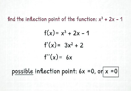
Set f’’(x) equal to 0 to find the candidate inflection points. Solving f’’(x) = 0 only gives you the candidate inflection points. These are the x-values of the possible inflection points for the function. You still need to test the points on the second derivative to make sure it changes concavity, or switches its sign from positive to negative or negative to positive. Set f ′ ′ ( x ) = 6 x {\displaystyle {\begin{aligned}f^{\prime \prime }(x)&=6x\end{aligned}}} {\displaystyle {\begin{aligned}f^{\prime \prime }(x)&=6x\end{aligned}}} equal to 0. 6 x = 0 x = 0 {\displaystyle {\begin{aligned}6x&=0\\x&=0\end{aligned}}} {\begin{aligned}6x&=0\\x&=0\end{aligned}}
Checking the Candidate Inflection Points
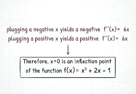
Plug a value higher and lower than the inflection point into f’’(x). To check if the second derivative changes signs, select 1 value that is greater than the candidate point and 1 value that is less than it. Then, plug each value into the second derivative. If the sign of the second derivative is different for both values, the candidate inflection point is an inflection point. If the sign doesn’t change, the candidate point is not an inflection point. In our example function of f ( x ) = x 3 + 2 x − 1 {\displaystyle f(x)=x^{3}+2x-1} f(x)=x^{{3}}+2x-1, the second derivative is f ′ ′ ( x ) = 6 x {\displaystyle f^{\prime \prime }(x)=6x} {\displaystyle f^{\prime \prime }(x)=6x} and the candidate inflection point is x = 0. {\displaystyle x=0.} x=0. Choose a value where x > 0 {\displaystyle x>0} {\displaystyle x>0} and x < 0. {\displaystyle x<0.} {\displaystyle x For this example, we’ll use x = 1 {\displaystyle x=1} x=1 and x = − 1 {\displaystyle x=-1} x=-1 as test values. Plug x = 1 {\displaystyle x=1} x=1 into f ′ ′ ( x ) = 6 x . {\displaystyle f^{\prime \prime }(x)=6x.} f^{{\prime \prime }}(x)=6x. f ′ ′ ( 1 ) = 6 ( 1 ) = 6 {\displaystyle f^{\prime \prime }(1)=6(1)=6} {\displaystyle f^{\prime \prime }(1)=6(1)=6} Plug x = − 1 {\displaystyle x=-1} x=-1 into f ′ ′ ( x ) = 6 x . {\displaystyle f^{\prime \prime }(x)=6x.} f^{{\prime \prime }}(x)=6x. f ′ ′ ( − 1 ) = 6 ( − 1 ) = − 6 {\displaystyle f^{\prime \prime }(-1)=6(-1)=-6} {\displaystyle f^{\prime \prime }(-1)=6(-1)=-6} f ′ ′ ( x ) {\displaystyle f^{\prime \prime }(x)} f^{{\prime \prime }}(x) changes signs when you plug in a lower x {\displaystyle x} x and a higher x {\displaystyle x} x than x = 0. {\displaystyle x=0.} x=0. Therefore, x = 0 {\displaystyle x=0} x=0 is an inflection point of the function f ( x ) = x 3 + 2 x − 1. {\displaystyle f(x)=x^{3}+2x-1.} f(x)=x^{{3}}+2x-1.
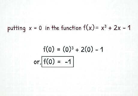
Substitute the inflection point into the original function to get its y-value. While you now know the x-value of the inflection point, you don’t know where it is on the y-axis. Simply go back to the original function and plug in the inflection point to get its y-value. The original function is f ( x ) = x 3 + 2 x − 1 {\displaystyle f(x)=x^{3}+2x-1} f(x)=x^{{3}}+2x-1 and the inflection point is x = 0. {\displaystyle x=0.} x=0. f ( 0 ) = ( 0 ) 3 + 2 ( 0 ) − 1 = − 1. {\displaystyle f(0)=(0)^{3}+2(0)-1=-1.} f(0)=(0)^{{3}}+2(0)-1=-1.
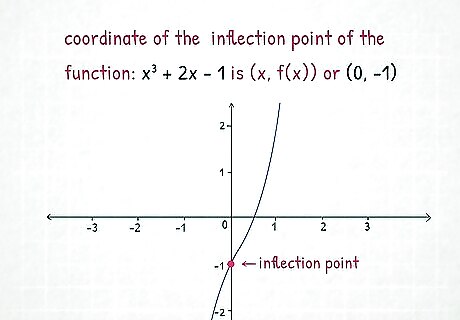
Evaluate the function to find the inflection point’s coordinates. The coordinate of the inflection point is denoted as ( x , f ( x ) ) . {\displaystyle (x,f(x)).} (x,f(x)). In our example, the coordinates of the inflection point are ( 0 , − 1 ) . {\displaystyle (0,-1).} (0,-1).
Troubleshooting Common Problems
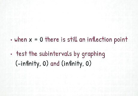
Check the concavity of every candidate inflection point. Oftentimes, people assume there’s no inflection point when the candidate point is x = 0 {\displaystyle x=0} {\displaystyle x=0}. However, this isn’t true. Remember, 0 can be graphed, so if you get 0 as your candidate point, it might be an inflection point. For example, if you get a candidate inflection point where x = 0 , {\displaystyle x=0,} {\displaystyle x=0,} make subintervals at ( − i n f i n i t y , 0 ) {\displaystyle (-infinity,0)} {\displaystyle (-infinity,0)} and ( 0 , i n f i n i t y ) . {\displaystyle (0,infinity).} {\displaystyle (0,infinity).} If the sign changes for the test values you choose at each interval, the inflection point is at 0. If you have inflection points at x = − 1 {\displaystyle x=-1} {\displaystyle x=-1} and x = 7 , {\displaystyle x=7,} {\displaystyle x=7,} you test the x values at ( − i n f i n i t y , − 1 ) , ( − 1 , 7 ) , {\displaystyle (-infinity,-1),(-1,7),} {\displaystyle (-infinity,-1),(-1,7),} and ( 7 , i n f i n i t y ) . {\displaystyle (7,infinity).} {\displaystyle (7,infinity).} Plugging in your test values into the second derivative at each interval tells you if both x = − 1 {\displaystyle x=-1} {\displaystyle x=-1} AND x = 7 {\displaystyle x=7} {\displaystyle x=7} are inflection points.

Include candidate points where the derivative is undefined. When you find possible inflection points, you have to look for instances where the second derivative equals 0 and where the second derivative is undefined. If you only look for points where the second derivative is 0, you might miss inflection points where the function is undefined.

Analyze the second derivative, not the first one. When you’re finding inflection points, you only consider the second derivative. If you set the first derivative equal to 0, your answer will give you extremum points instead. For example, if you are finding whether or not h ( x ) = x 2 + 4 x {\displaystyle h(x)=x^{2}+4x} {\displaystyle h(x)=x^{2}+4x} has an inflection point, you consider h ′ ′ {\displaystyle h^{\prime \prime }} {\displaystyle h^{\prime \prime }}, NOT h ′ {\displaystyle h^{\prime }} {\displaystyle h^{\prime }}. This is because h ′ ′ {\displaystyle h^{\prime \prime }} {\displaystyle h^{\prime \prime }} is the second derivative, while h ′ {\displaystyle h^{\prime }} {\displaystyle h^{\prime }} is the relative minimum point (which you aren’t looking for here).
Using a Scientific Calculator to Find Inflection Points
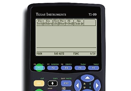
Head to your “Plots” function on your calculator. It’s easy to use a scientific calculator to find inflection points. On most scientific calculators, just press the “diamond” or the “second” button, then click F1. This takes you to your Y plots where you can enter up to 7 functions. This is true on both the TI-84 and the TI-89, but it may not be the exact same on older models.
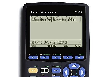
Enter the function into y1. Clear out any remaining functions you had in your y plots. Then, type in the function after the equal sign. Remember to keep any parentheses involved in the function so your answer is correct. For example, the function might be y 1 = x 3 − 9 / 2 x 2 − 12 x + 3 {\displaystyle y1=x^{3}-9/2x^{2}-12x+3} {\displaystyle y1=x^{3}-9/2x^{2}-12x+3}
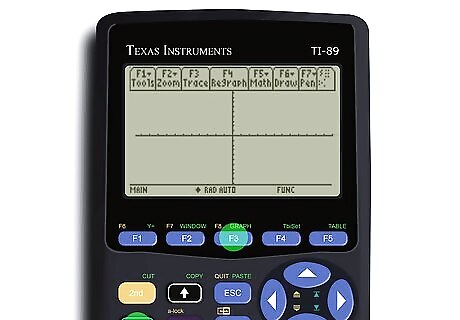
Click “graph.” On most calculators, you press the “diamond” or “second” button then click F3. If you have to adjust your window on the calculator, hit “diamond” or “second” and press F2. Then, select “standard zoom.” Don’t worry if your screen doesn’t show the whole graph just yet—you will adjust the zoom later.
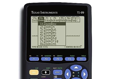
Adjust the window until you see the whole graph. When you open up the graphing window, you might not see the entire curve of your graph. If that’s the case, click the “diamond” or “second” button, then open up F2 for zoom again. Simply increase or decrease your minimum and maximum axis to get the graph to fit inside the window. It might take a little adjustment and back-and-forth to find your graph.
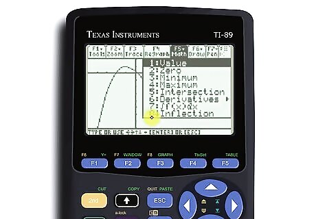
Click “Math,” then “Inflection.” Hit the “diamond” or “second” button, then select F5 to open up “Math.” In the dropdown menu, select the option that says “Inflection.” This is—you guessed it—how to tell your calculator to calculate inflection points.
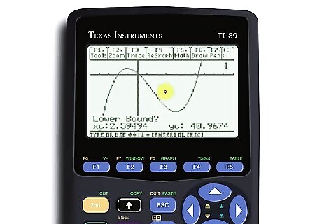
Place the cursor on the lower and upper bound of the inflection. Your calculator will give you a message saying “Lower?” Move the arrows on your calculator until the cursor is to the left of the inflection point. Then, your calculator will ask “Upper?” Move your cursor so it’s to the right of the inflection point. To get your inflection point, hit “Enter.” This is how you get your calculator to guess where the inflection point is. Now you have your answer!


Comments
0 comment