views
Using Conditional Formatting
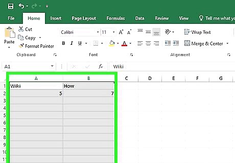
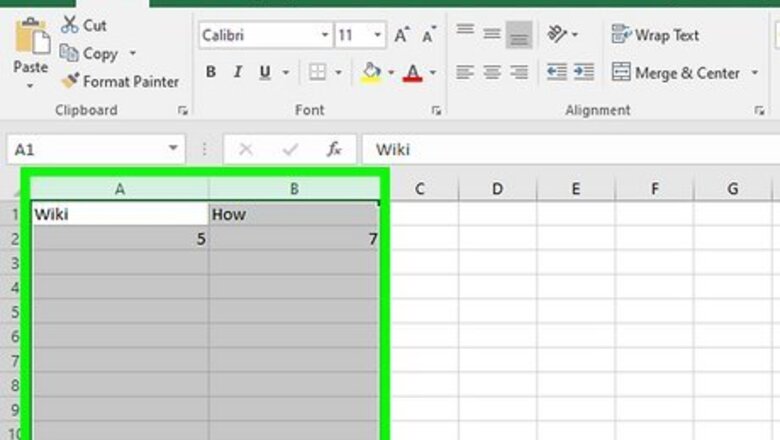
Select the columns you would like to compare. Using conditional formatting in Excel will allow you to automatically highlight any matching values across multiple columns. Click and drag your mouse over the columns you would like to compare. If the two columns are not side by side, simply hold down Ctrl and select whichever columns you need.
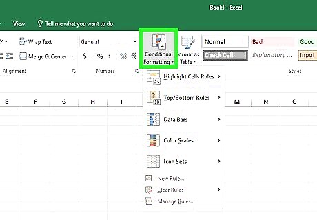
Click Conditional Formatting from the "Home" tab. This will open up a drop-down menu with various additional options.
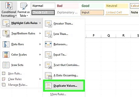
Select Highlight Cells Rule and then Duplicate Values. This setting tells Excel that you want your conditional formatting to detect values that are duplicated (i.e., match) across your selected columns.
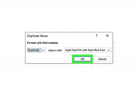
Click OK on the pop-up window. After selecting your conditional formatting settings, Excel will show you a pop-up window. Ensure the window reads Duplicate in the left-hand box, and click "OK." The other box in the pop-up window allows you to change the colors Excel uses to indicate duplicates. The default is "Light Red Fill with Dark Red Text", but you may choose whichever you prefer.
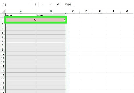
Identify the matching values. Excel will now highlight any duplicates with the formatting you chose in the previous pop-up box. Look for this colored formatting and identify any matches. Using conditional formatting to find matching values is a handy way to find matches that may not be in the same row.
Using VLOOKUP

Create a third column next to your two columns of data. The VLOOKUP function involves using a specific formula to find matching values. You'll need a third column to input the formula and display any matches.
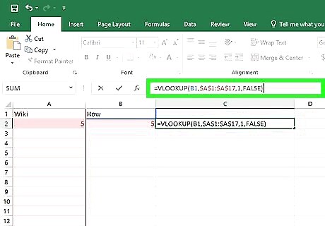
Enter the VLOOKUP formula into the first row of the third column. Assuming your data begins from the top-left corner of your spreadsheet, the formula is as follows: =VLOOKUP(B1,$A$1:$A$17,1,FALSE). The "17" in the formula indicates 17 rows of data. Change the number to fit however many rows of data you have. The "FALSE" value at the end of the formula is what tells Excel to look for an exact match in value. Replace it with "TRUE" to search for the nearest match that is less than or equal to the corresponding data point (represented in this case by B1). Just entering "=VLOOKUP" in Excel will pull up the full formula, which you can reference in populating each field with the necessary info.
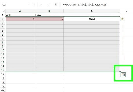
Copy the VLOOKUP formula all the way down. Drag down from the corner of the first box to your final row of data to copy the formula. Excel will automatically change the first value to the corresponding data point in that row.
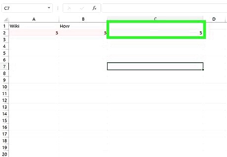
Look for matching values in your third column. If there are any matching values, they will display as a number in your spreadsheet's third column. If there are no matching values, the VLOOKUP formula will simply turn up "#N/A".
Using a TRUE/FALSE formula
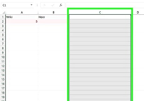
Create a third column next to your two columns of data. This method involves using a specific formula to find matching values. You'll need a third column to input the formula and display its results.
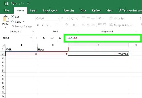
Enter the TRUE/FALSE formula into the third column. Assuming your data begins from the top-left corner of your spreadsheet, the formula is as follows: =A1=B1.
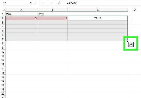
Copy the formula all the way down. Drag down from the corner of the first box to your final row of data to copy the formula. Excel will automatically change the values to the corresponding data points in that row.
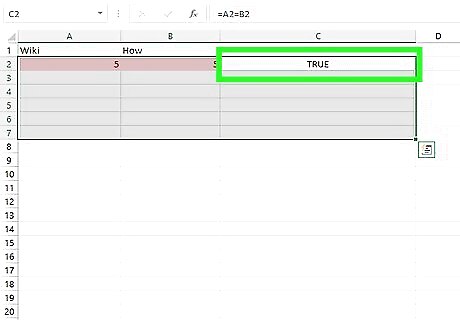
Look for a "TRUE" or "FALSE" assessment in the third column. Matching values will turn up a "TRUE" value. If there is no match, the box in the third column will read "FALSE."










Comments
0 comment