views
Creating Columns
Get familiar with Excel. Excel is a spreadsheet software program that allows users to manage data and perform calculations with formulas. Excel spreadsheets are organized by rows and columns. You can install a desktop version of Excel on your Mac or PC. Or, you can use a free online app for your smartphone, tablet or computer. Each of these versions functions a little bit differently. Excel has been in existence for many years, and every year or so, Microsoft releases a new, updated version. Each of these versions also works a little bit differently. In Excel, rows run horizontally and are ordered by number. Columns run vertically and are ordered by letter. Each box where a row and column intersect is called a cell. The cell is named according to its row and column. For example, a cell in the fifth row of column D is named D5 (column D, row 5). Understand the difference between a worksheet and a workbook in Excel. A worksheet is a single spreadsheet. A workbook is an Excel file that contains one or more spreadsheets. Each worksheet in an Excel workbook is in a separate tab. By default, new Excel workbooks have three tabs. You can add more if needed. To make a basic check register, you only use one tab. To create a function for categorizing expenses in a check register, you will use two tabs.
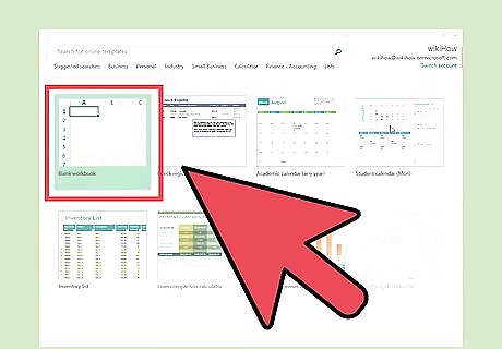
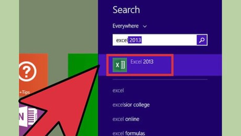
Open a blank Excel spreadsheet. How you open the spreadsheet differs depending on the type of computer and operating system you are using. On a PC with an operating system older than Windows 7, begin by clicking on the start menu in the lower left hand corner of your desktop. From the popup menu, click on Programs. From the next popup menu, click on Microsoft Office. Then click on Microsoft Office Excel. At this point you will have a blank excel spreadsheet on your desktop. On a PC with Windows 7 or newer, click on the Windows icon in the lower left hand corner of your screen. Then click on the Microsoft Excel tile to open Excel. You will see a page with your recent files listed on the left and template options for new documents on the right. Click on the first template option, Blank Workbook, to open a new Excel spreadsheet. To open Excel on a Mac, click on Excel in the dock. Click “File” in the menu bar. Click “Open” and then click “New.” This will bring you to a new, blank spreadsheet.
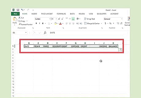
Create column labels. Use labels that you would find in an ordinary paper check book register. Create columns for the date, check number, the payee and a description or memo. After that, create columns for debits (which are payments or withdrawals), credits (which are deposits) and the balance forward. Enter the word “DATE” in cell B1 (column B, row 1). This is where you will enter the date of the transaction. Move one cell to the right to cell C1 (column C, row 1). Type “ITEM #”. Here you will enter the check number or the type of transaction, such as “ATM” or “deposit.” Move one cell to the right to cell D1 (column D, row 1). Type “PAYEE.” This is the person to whom a check was made payable or to whom money was paid. Move one cell to the right to cell E1 (column E, row 1). Type “DESCRIPTION.” Record any details you want to remember about the transaction. Move one cell to the right to cell F1 (column F, row 1). Type “DEBIT.” This is where you record money that leaves your account, also known as outflow. Move one cell to the right to cell G1 (column G, row 1). Type “EXPENSE CATEGORY.” You will leave this blank for now. Options for this column will be created in a later step. Move one cell to the right to cell H1 (column H, row 1). Type “CREDIT.” This is where you record money coming into your account, also known as inflow. Move one cell to the right to cell J1 (column J, row 1). Type “INCOME CATEGORY.” As with the expense category column, options for this column will be created in a later step. Move one cell to the right to cell K1 (column K, row 1). Type “BALANCE.” This is the current amount in your account after all transactions have been recorded.
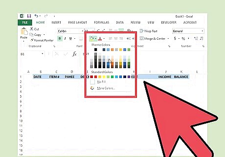
Format column labels. To make the column labels easy to read, format them so they are in bold font and give the row of register labels a different background color. To do this, first you select the range of cells that you want to format. Then you select the formatting options. Find the formatting options in the “HOME” tab of the toolbar ribbon. When you open a new workbook, the “HOME” tab is open by default. Select cell B1 (DATE) and drag the cursor across all of the labels, through cell K1 (BALANCE). In the upper left hand corner of the toolbar, click on the “B” for the bold formatting option. To change the color of the background, click on the paint bucket icon to see the palette from which you can select your background color.
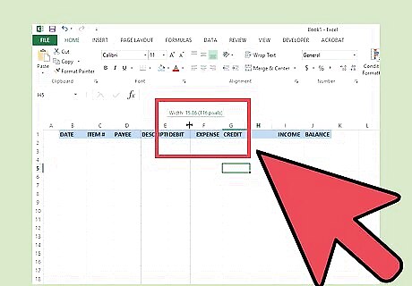
Resize some of the columns. The default size of some of the columns will likely be too small to hold the data you will put in them. For example, the “PAYEE” and “DESCRIPTION” columns could hold long names or lengthy memos. Also, column A, which has no data and is just a spacer, should be very narrow. Click the header for column A to select the whole column. In the upper right hand corner of the toolbar in the “HOME” ribbon, click on the “FORMAT” button. From the drop down menu, click on “Column Width.” Enter the number 2 and click on “OK.” Now column A is very narrow. Widen column D, “PAYEE.” Select column D by clicking on the header. Hover the cursor over the border between columns D and E. The cursor will change from the arrow to the resizing cursor. The resizing cursor looks like a cross with arrows. When you see the resizing cursor, left-click and drag your mouse to the right to make the column as wide as you want it to be. Repeat the same procedure to widen column E, “DESCRIPTION.”
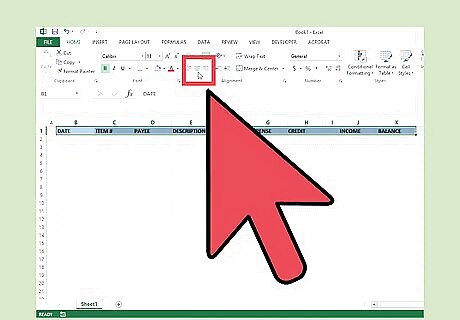
Center the register labels. Select the entire first row by left-clicking on the number 1 on the left border of the page. In the upper left hand side of the toolbar on the “HOME” ribbon, click on the “center” formatting button. This action centers all of the data in the selected cells. You will notice that the column labels are now centered in their cells.
Formatting Cells
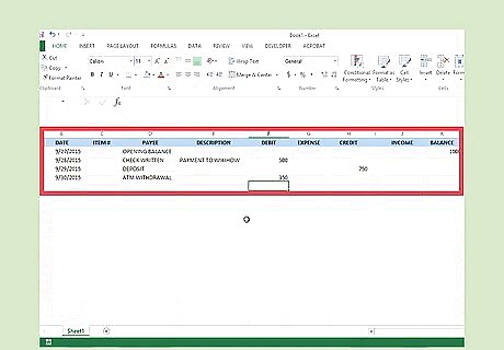
Input some test data. In order to see the formatting changes you make, enter four rows of data into the cells. Begin with the opening balance, and then enter three more transactions. In cell B2, add a date for the opening balance, for example 9/27/15. In cell D2, which is the “PAYEE” column, type “Opening Balance.” In cell K2, which is the “BALANCE,” type the amount of money you have in your account as of the date you entered in cell B2. Add three more transactions. Try to have a mix of debits (such as checks written or ATM withdrawals) and credits (such as deposits). Notice the inconsistent formatting of the numbers in the cells. The date column may be formatted to read “9/27/2015” or “27-Sept.” The columns in which you entered dollar amounts may have the wrong number of decimal points. Formatting will clean all of this up.
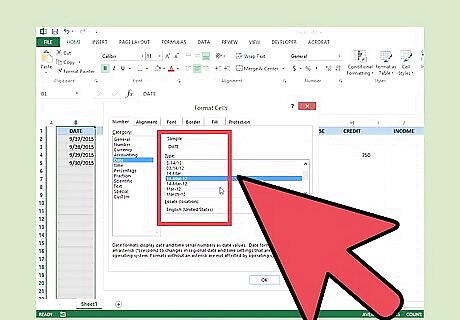
Format the dates. Make this column display the dates in a consistent way. Excel provides different options for formatting the date. Select the one that you prefer. Click on the header for column B, “DATE.” This selects the entire column. Right-click on the column, and select “Format Cells.” The “Format Cells” window will appear. Select the “Number” tab. Under “Category” choose “Date.” Select the format you desire for the date and click on “OK” in the bottom right corner of the window. While this column is still highlighted, center the data in these cells by clicking on the “center” icon in the upper left hand corner of the toolbar in the “HOME” ribbon.
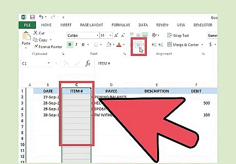
Format the “ITEM #” column. The data in this column should be centered. Highlight all of column C by clicking on the header for the column. Click on the “center” icon. Notice the test data you entered in this column. It should be centered in the cells. Check the formatting for columns D and E, “PAYEE” and “DESCRIPTION.” By default, Excel formats cells so that the data is aligned to the left. This should work well for these columns. Double check the sizing of the columns. Now that you have some data in these cells, adjust the column width to make the columns wider or narrower if necessary.
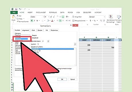
Format the currency in columns F, H and K, “DEBIT,” “CREDIT” and “BALANCE FORWARD.” The currency should have 2 decimal points. You can choose to show the dollar sign if you desire. You can also make your debits appear in red font if you want. Select column F. Right-click on the column and select “Format Cells.” The “Format Cells” window will appear. In the “Number” tab, select “Accounting. “ Choose “2” in the “Decimal places” option. Select the dollar sign in the “Symbol” option. Repeat for columns H and K. To make your debits appear red, click on the header for column F to select the entire column. Right click on the column and select “Format Cells.” When the “Format Cells” window appears, select the “Font” tab. In this tab, click the down arrow next to the “Color” option. From the palette, click on red.
Creating Formulas
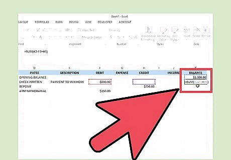
Create a formula to calculate a running balance. Insert a formula into column K that does the math to calculate the running balance. Note that you did not need a formula in cell K2. This is where you entered your opening balance. Click on cell K3. Now click on the formula bar at the top of the spreadsheet. This is where you will type in the formula that tells the cells to perform a calculation. Type the formula =SUM(K2-F3+H3). This tells the spreadsheet to take our opening balance (cell K2), and subtract a debit if one exists (cell F3) and add a credit if one exists (cell H3). Suppose your opening balance was $200, and your first entry was a check you wrote for $35.00. The $35.00 is recorded as a debit in cell F3. The formula you entered in cell H3 takes the opening balance and subtracts the debit, leaving you with a balance of $165.00.
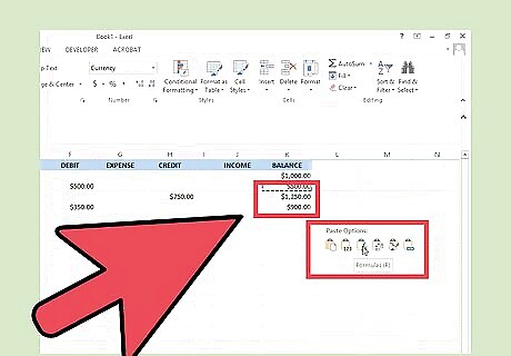
Copy the formula. Select cell K3. Right-click and select “Copy.” Select cells K4 and K5. Right-click and select “Paste.” The formula is now copied into these cells. You should see that the running balance has been calculated in column K for all the rows of test data that you entered.
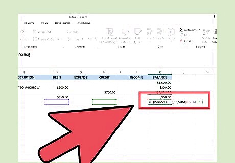
Create a conditional formula to clean up the running balance column. You could copy the above formula into cell K6. But since you haven’t entered any data in this row, the running balance from cell K5 will also appear in cell K6. To clean this up, create a conditional formula that leaves the cell blank if no transactions have been entered, but displays a balance if they have been entered. In cell K6, enter the formula =IF(ISBLANK(B6),"",SUM(K5-F6+H6)). This tells Excel that if cell B6, in the “DATE” column, is blank, then cell H6 should be blank. But if cell B6 is not blank, then the balance should be calculated.
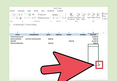
Extend the formula with AutoFill. The AutoFill automatically fills in formulas in adjacent cells so you won’t have to enter the “BALANCE” formula over and over again. Find the AutoFill handle in the active cell. Observe the small, dark square in the bottom right corner of the active cell. Hover over it and the cursor will change to the AutoFill cursor, which looks like a thin plus sign. Click on cell K6. Hover over the AutoFill handle and the cursor will change to the thin plus sign. Left-click and hold the AutoFill handle. Drag the cursor down to cell K100 (column K, row 100). The formula has now been copied into all of the cells in column K through row 100. The row and column numbers in each cell have been automatically adjusted so the formula calculates correctly.
Adding Categories
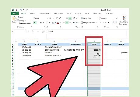
Categorize transactions. Create categories of transactions to keep track of how you spend your money and the types of income. Categories could be related to income taxes, such as property taxes or charitable giving. You could also use the categories to create a charts to easily visualize financial activity in your account.
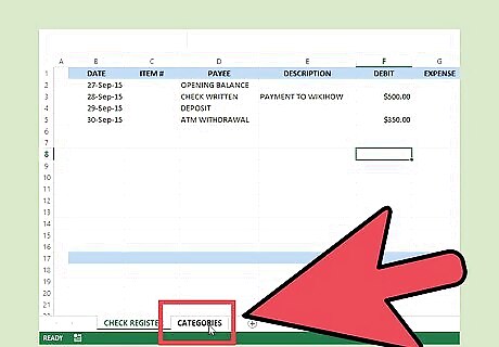
Create a “Categories” tab. This is where you will store all of the potential income and expense categories for your check register. Rename one of the tabs in your workbook “Categories.” Double click on the current title of the tab to highlight the name. The current name will be something like “sheet2” or “sheet3.” When the name of the sheet is highlighted, you can type in the new name of the tab. Type “Categories.” . In cell B4, type the word “Categories.” Format the cell to have bold font and change the alignment to center.
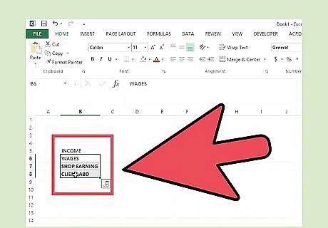
Create income categories. In cell B5, type “*** Income ***”. Think of all of the categories of income you have or may utilize in the future. In cell B6 and continuing downward, enter all of your income categories. The most common income category would be “Wages.” You might need multiple wage categories if you have more than one job. Other income categories you might want to include depend on your financial circumstances. If you own stock, create a category for “Dividends.” If you receive child support, create a category for that. Other categories to add include “Interest Income,” “Gifts” and “Miscellaneous.”
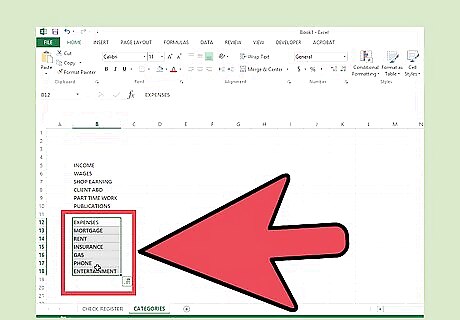
Create expense categories. Leave a cell blank under your last income category. Move one cell down and type “*** Expenses ***”. Enter all of the expense categories under this section heading. Be as broad or as narrow as you wish with your expense categories. Expense categories might include “Mortgage,” “Rent,” “Insurance,” “Car Payment,” “Gas,” “Electricity,” “Phone” and “Entertainment.”
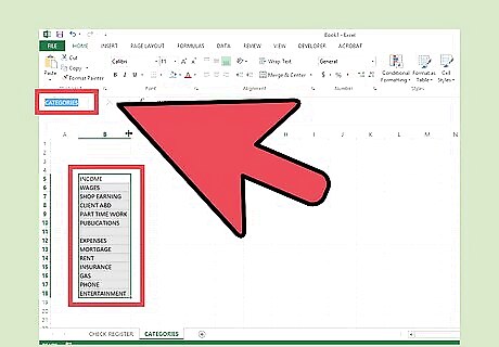
Name the range of cells containing your categories. Select cell B5. Highlight from cell B5 all the way down through all of your income and expense categories. Find the cell name box in the upper left hand corner of the window. It is to the left of the formula box. It will say “B5,” which is the name of the first cell in the highlighted range. Click on the cell name box and type “Categories.” This names the range of cells so you can use it in your check register.
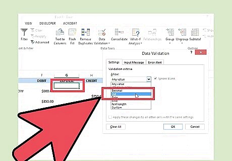
Use the expense and income categories in the check register. Go back to the tab where you created the check register. You will now add drop down menus to the “EXPENSE CATEGORY” and “INCOME CATEGORY” columns you created. In the check register tab, select cell G2. This is the first cell in the “EXPENSE CATEGORY” column. On the toolbar, select the “DATA” ribbon. Click on the “Data Validation” button. Select “Data Validation” from the drop down menu. This will open the “Data Validation” window. In the “Settings” tab of the “Data Validation” window, look for the “Allow” drop down box. Click on the down arrow and select “List.” Under “Source” enter “=Categories.” Click OK. You will now see a little arrow next to cell G2. Click on the arrow to see the list of categories. Click on the appropriate category for the transaction in that row. Using AutoFill, copy the formula from cell G2 all the way down to cell G100. Go to cell J2 to repeat the process in the “INCOME CATEGORY” column.
Protecting Check Register
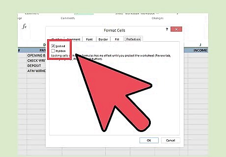
Lock the cells with formulas and protect the worksheet. Protecting the worksheet means that data in locked cells cannot be overwritten. This way you don’t have to worry about the balance forward being incorrectly calculated because the formula was accidentally changed. You can also create a password to further protect your check register from other users. Just make sure it's something that is easy for you to remember, or you write it in a secure place; if you forget the password you will be unable to access the worksheet.
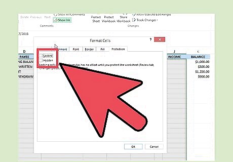
Unlock cells. By default, once a worksheet is protected, all of the cells become locked. So to begin, you need to unlock the cells into which data will entered even after the worksheet is protected. Select cells B2 through J100. This is all of the cells in all of the columns of the check register except the last column, K, which is the “BALANCE” column. You are going to need to be able to enter data in these cells even after the worksheet is protected. Right-click inside the selected range of cells. Select “Format Cells.” In the “Format Cells” window, select the “Protection” tab. Uncheck the box that says “Locked” and click OK.
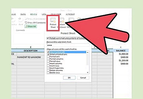
Activate “Protection” for the worksheet. Once “Protection” is activated, this means that all cells which remained locked, including the cells in column K, “BALANCE,” cannot be overwritten. Go to the “REVIEW” ribbon on the toolbar. Click on “Protect Sheet.” The “Protect Sheet” window will appear. If you want to password protect your worksheet, add it here. If not, leave this field blank. Click on OK. Your check register is no protected.
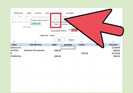
Unprotect your worksheet to change locked cells. If you decide to change formulas in locked cells, you can reverse this process. Go to the “REVIEW” ribbon on the toolbar. Click on “Unprotect Sheet.” The “Unprotect Sheet” window will appear. Click on OK.


Comments
0 comment