How to Calculate a Balloon Payment in Excel

Calculating a Balloon Payment in Excel

Gather the details of your proposed balloon payment loan. You'll need to know your annual interest rate, loan amount (the principal), the duration of your loan (in years), and your monthly payment. These can be found on your loan agreement. Alternately, you can enter your own values for a loan agreement you think you could get. Be sure to research the prevailing interest rate on your loan type for your creditworthiness. You can get the monthly payment amount from there by reading and following the directions at how to calculate loan payments.

Open a new worksheet in Excel. Open Excel on your computer and choose to open a new, blank workbook. The program should then display a blank worksheet. This will be your workspace for calculating your balloon payment.

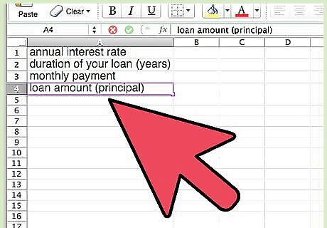
Create labels for your variables. Enter your variables' names in the cells from A1 down to A4 as follows: annual interest rate, duration of your loan (years), monthly payment, and your loan amount (principal). This will ensure that you don't mix up any values if you change your variables later.

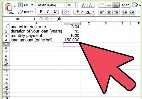
Enter the variables for your loan. Fill in your variables in the adjacent cells to your labels. These will be cells B1 to B4. Check again to make sure you've put the right variables into each cell, because your calculations will depend on this. For example, consider the following variables: An annual rate of 4% would be entered into B1 as 0.04 A 15-year loan would be entered into B2 as 15. A monthly payment of $1000 would be entered into B3 as -1000. Be sure this is entered as a negative number. This is how Excel recognizes payments. A loan amount of $150,000 should be entered into B4 as 150,000.

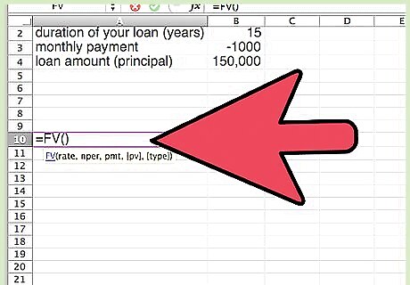
Set up your equation. The equation used to calculate your payment payment is the future value function. This is denoted in Excel with the symbol "FV." It can be either typed in manually to a nearby cell by typing "=FV(" or found in the functions tab under financial functions. Either way, when you type it into a cell, the function will prompt you for variables as follows: =FV(rate, nper, pmt, [pv], [type]).

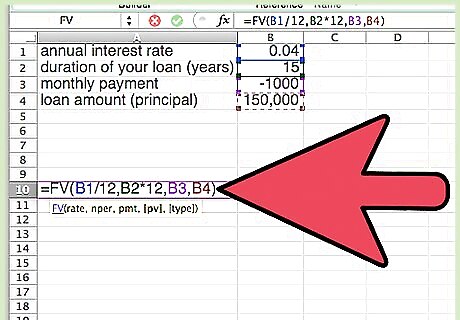
Enter your variables. Each variable will be linked from your variables you've already entered on your worksheet. However, some changes must be made to some of the variables when they are entered. Additionally, they must be entered in the right order. Enter your variables as follows: The prompt "rate" is asking for your periodic interest rate. That is, your monthly interest rate. When prompted, after typing "=FV(", click on cell B1, where your rate should be. Then, type "/12" to divide your annual rate by 12 and find your monthly interest rate. The program will now calculate this for you in your equation. Enter a comma to move on to the next variable. If your payments are quarterly, divide by 4 instead of by 12. For semi-annual payments, divide by 2. Assuming monthly payments, your equation should now look like this: =FV(B1/12, The prompt "nper" is asking for the total number of payments. Here, you'll want to multiply the duration of your loan by 12 to find the total number of monthly payments made on the loan. When prompted, click on B2 and then type *12 to multiply it within the equation. Enter a comma to move on to the next variable. Multiply by 4 for quarterly payments or 2 for semi-annual payments. Assuming monthly payments, your equation should now look like this: =FV(B1/12,B2*12, The prompt "pmt" is simply asking for your monthly payments as entered in B3. Simply click on B3 when prompted or type it into the equation. Enter a comma to move on to the next variable. Your equation should now look like this: =FV(B1/12,B2*12, B3, The fourth prompt, "[pv]," is just asking for the principal, or loan amount. Simply click on B4 when prompted. You can then close off the equation with a closing parenthesis. The last variable, "[type]," is unnecessary here. Your final equation should be as follows: =FV(B1/12,B2*12,B3,B4)

Press enter to solve your equation. Check that you've entered everything correctly and that your equation doesn't contain any errors or unnecessary numbers. The program will return your answer in the same cell where you entered the formula.

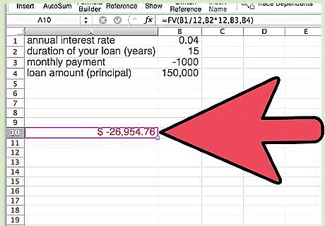
Review your answer. The answer will be returned as a negative number if you've entered everything correctly. This simply means that it is a payment and not a return. The number displayed will be the balloon payment due at the end of your loan. If the number is positive, this means either that you've entered your data incorrectly or that you don't have a balloon payment loan. Using the variables in this example, a balloon payment of $26,954.76 will be due at the end of the loan's term.

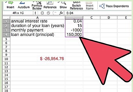
Adjust the variables, if desired, to reflect a different interest rate or payment amount. This will allow you to calculate the effect of a better rate, making a higher monthly payment, or extending the length of your loan.

Calculating Payments on a Balloon Payment Loan

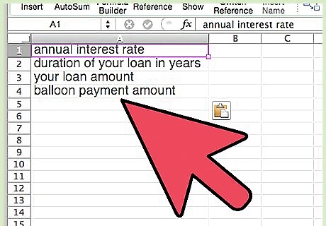
Collect your information. Calculating your payments in this way will allow you to see how much you would pay per month with a given balloon payment at the end of the life of the loan. To find this information, either consult your loan agreement or estimate this information as best you can. Remember, you can always change this information to multiple different values to estimate payments on different loans. You'll need the following information: your annual interest rate, the duration of your loan in years, your loan amount, and your balloon payment amount.

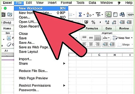
Open a new worksheet in Excel. Start by opening Excel on your computer. Then, open a new, blank workbook and begin your work on the worksheet that comes up.

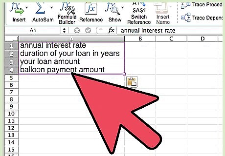
Enter labels for your variables. In the first column, column A, enter the names for the variables you will be using. It's easiest if you enter them as follows, from top to bottom: your annual interest rate, the duration of your loan in years, your loan amount, and your balloon payment amount. If entered correctly, this information will be in cells A1 through A4.

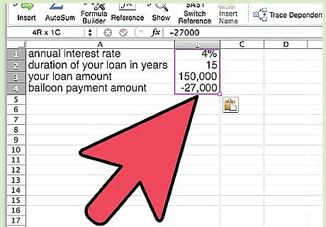
Input your variables. Type your loan information into the appropriately-labeled spaces next to your variable names. If entered correctly, they should be entered as follows: Your annual interest rate, for example 4%, should be entered in cell B1. Be sure to include the percent sign. Your loan duration, for example 15 years, should be entered in cell B2 as a simple number. In this case, you would just enter 15. Your loan amount, also called the principal, should be entered into cell B3. For example, for a loan amount of $150,000, you would enter 150,000. Excel will assume this is an amount of money; no need to enter the dollar sign. Enter your balloon amount into cell B4. This should be a negative number, as it is a payment. For example, for a $27,000 balloon payment, you would enter -27,000.

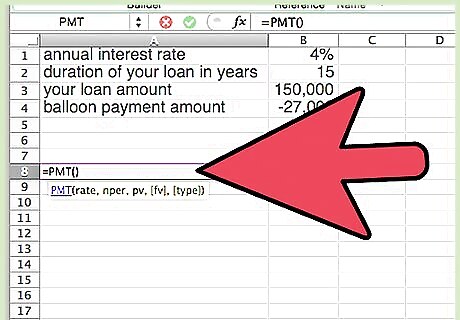
Set up your equation. The function that will be used here in the payment function, abbreviated by Excel as PMT. To enter this equation, find a nearby empty cell and type "=PMT(". The program will then prompt you for variables like this: =PMT(rate, nper, pv, [fv], [type]).

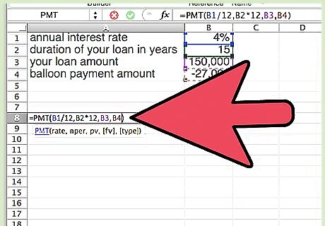
Input your variables into the equation. Additional changes will have to be made to your entered variables within the PMT function. When prompted, enter the variables as follows: For the "rate" prompt, you'll need your periodic rate instead of your annual rate. This means dividing your annual rate in cell B1 by the number of payments per year on your loan. For monthly payments, divide by 12, for quarterly payments by 4, and for semi-annual payments by 2. Enter a comma to move to the next variable. Assuming monthly payments, your equation should now look like this: =PMT(B1/12 For the "nper" prompt, enter your loan duration in cell B2. However, like the rate prompt, this will need to be adjusted to the total number of payments. For monthly payments, multiply by 12, for quarterly by 4, and for semi-annual by 2. Enter a comma to move to the next variable. Assuming monthly payments, your equation should now look like this: =PMT(B1/12,B2*12, Enter your last two variables, in B3 and B4, for the "pv" and "[fv]" prompts, respectively. Be sure to enter a comma after B3. Then, close the equation with a closing parenthesis mark. Your finished equation should look like this: =PMT(B1/12,B2*12,B3,B4)

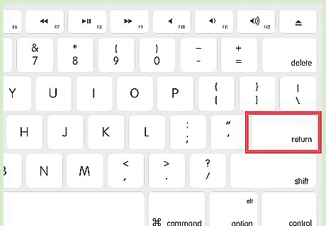
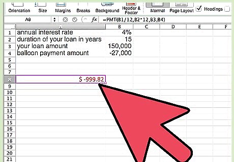
Solve your equation. Press enter. Your result should be displayed in the cell where you entered your equation. It will be a red, negative number. Again, this simply means that this a payment. If it is not a negative number, you've entered some information incorrectly or your loan is not a balloon payment loan. In the example, the program would return a monthly payment of $999.82.

Edit the numbers. If you are comparing multiple loans, save this payment figure elsewhere in the worksheet and enter information from your other loans. This will allow you to compare payments from different loan amounts, interest rates, durations, or balloon payments.